Week 2 Notes
Note
Keep an eye weekly pages as they might be updated throughout the week.
Week 2 Overview
Welcome to week 2! Hopefully by now you have all settled in to the structure and organization of this course. At this point, you should have at least a basic understanding of what is required of you for assignment 1. If not, head over to the assignment overview page and carefully read through the requirements. If any of requirements sound unfamiliar to you, you will want to thoroughly explore the lecture and materials provided below.
- The recorded lectures for this week will cover the following topics:
You might also take a look at the lab schedule for week 2 and see if any of the topics align with your learning needs.
See you in class!
Lecture Materials
Recorded Lectures
Modules
In upcoming assignments, you will be required to start organizing your code a bit more than you have for a0 and a1. One way to organize code is to divide it into multiple .py files, which when imported to another file, are called modules. In this lecture, we’ll discuss strategies for importing modules and organizing and creating your own.
Lecture Recording
Lecture Notes
The code that we write to create a program in Python is stored in plain text files. Aside from some common conventions such as file extensions (.py), syntax, and indentation, Python files are no different then any other plain text file that you might write. So far, you have probably written most of your Python programs in a single file with a .py extension. Generally speaking, this is a good practice. Having all of your code in a single file simplifies things quite a bit. When all of your code (and tests!) is in one location you don’t have worry about connecting multiple files. However, as your programs grow in complexity and size, you will discover that managing all of your code in a single file quickly turns into a time consuming challenge. So let’s turn to the lecture to learn how we can improve the readability and reuse of our code with modules.
In Python, a module is nothing more than a file with the .py extension. However, unlike the programs you have written so far, a module does not produce output when executed directly from the shell. Let’s take a look at the following example:
# basicmath.py

def add(a: int, b: int) -> int:
	result = int(a) + int(b)
	return result

def subtract(a: int, b: int) -> int:
	result = int(a) - int(b)
	return result
If we were to run this program, basicmath.py, on the shell we would not receive any output from the Python interpreter. We would, however, be able to call the modules functions directly:
>>> add(2, 5)
7
>>> subtract(9, 3)
6
If we attempt to call these functions before we load basicmath.py the interpreter will return a Traceback that tells us that ‘add’ (or ‘subtract’) is not defined. So what is the difference? Well, by executing the basicmath.py module first we have loaded it into our program, which in this case is the Python shell. The Python programs that we write in .py files, operate in much the same way. Let’s write a small program that makes use of the basicmath.py module:
# mathrunner.py

import basicmath

a = input("Enter your first value: ")
b = input("Enter your second value: ")

result = basicmath.add(a,b)
print(result)

result = basicmath.subtract(a,b)
print(result)
Notice that the first line of code is an import statement followed by the name of our basicmath python module. We don’t need to specify the .py extension as it is implied that we are importing Python files. So, in the same way that you “imported” the Path module into your program for a1, we are able to import python files that we write.
Scope
Another important convention to consider in this code is how the add and subtract functions are accessed. You will see that when the variables are passed to the basicmath functions, the name of the module must first be referenced. Python, as well as most programming languages, operate under a concept called scope. Scope refers to the availability of classes (we will cover these in more detail later in the quarter), functions, and variables at a given point of execution in a program. In the example above, notice how the variable result is used in the add and subtract functions of the basicmath module as well as the mathrunner program. We can reuse variable names in this way due to Python’s scoping rules. result is locally scoped to the add and subtract functions, meaning that it only exists in the moment that each of those functions is being called. Now, if we wanted to make use of result outside of the add and subtract functions, we could modify the basicmath program like so:
# basicmath.py

result = 0

def add(a: int, b: int) -> int:
	result = int(a) + int(b)
	return result

def subtract(a: int, b: int) -> int:
	result = int(a) - int(b)
	return result

def get_last_result() -> int:
	return result
# mathrunner.py

import basicmath

a = input("Enter your first value: ")
b = input("Enter your second value: ")

result = basicmath.add(a,b)
print(result)

result = basicmath.subtract(a,b)
print(result)

print(basicmath.get_last_result())
Which will output:
Enter your first value: 5
Enter your second value: 2
7
3
0
Wait, why is the value of result still zero? Well, even though the variable result is scoped outside of both functions, or global, Python still gives precedence to the local instance of result. So the add and subtract functions create a local instance of result while get_last_result, in absence of any instantiation of a local result instance, defers to the global instance of result. To use the globally scoped variable, we need to tell Python that is our intention:
# basicmath.py

result = 0

def add(a: int, b: int) -> int:
	global result
	result = int(a) + int(b)
	return result

def subtract(a: int, b: int) -> int:
	global result
	result = int(a) - int(b)
	return result

def get_last_result() -> int:
	return result
Which will output:
Enter your first value: 5
Enter your second value: 2
7
3
3
There we go! So by setting the scope of the result variable inside each function to global we change the scope from local to global, allowing us to store a value in a shared variable. So scope can be thought of as consisting at two levels: global and local. The Python interpreter assumes a local first stance when interpreting program code and when a local instance is unavailable it assumes global.
Important
Scope refers to the availability of a particular object in a program. That availability is interepreted locally first and then globally.
Definition Access
When writing modules that contain many functions performing many different types of operations you will find that you need some of those functions to perform operations within your module, but you might not necessarily want those functions to be called outside of your module. In programming terms, we describe these two types of functions as private and public. While some programming languages do provide modifiers for declaring this intention at the point of compilation, Python does not. Rather, all functions in Python are public by default. There is no way to prevent another program from calling functions in your module that should not be called!
To get around this feature, and the absence of such modifiers is considered a feature in Python, programmers have adopted some formal conventions for communicating intent. When writing functions that you don’t intend to be used outside your module, they should be prepended with a single underscore character. This convention is used for functions, constants, and classes in Python:
# Specifying private intent

def _myprivatefunction():

_myprivateconstant = "525600" # minutes in a year

class _myprivateclass():
We will be looking more closely at your use of naming conventions like private and public access as we move forward with assignments this quarter. Not only do we want to you to continue to adopt formal Python programming conventions, but thinking about access will help you to improve the structure of your modules. So start considering what operations in your program need to be conducted outside the scope of your module and more importantly, what code should not be accessed.
Namespaces
As your programs grow in size and complexity the importance of understanding scope will become increasingly relevant. Without the ability to scope the objects that we create, every Python programmer would have to create unique object names! Imagine if object naming behaved like Internet domain names, each one having to be recorded in a central registry to avoid duplicates. Through scope, and a convention called namespaces, most programming languages can avoid this unnecessary complication. A namespace is a dictionary-like collection of symbolic names tied to the object in which they are currently defined.
Namespaces are not a perfect solution, but they serve well to help programmers identify and differentiate the modules and programs that they write. It is important to avoid using known namespaces, particularly those that are used by Python’s built-in objects. For example, you should avoid creating an object named int or tuple because they already exist in every instance of a Python program. Imagine if we had named our basicmath module math, which is part of the standard library! To put it more concretely, what if we also had an add function in our mathrunner.py program? Namespaces allow us to differentiate between like named objects:
# mathrunner.py

import basicmath as m

def add(a, b):
	print(a + b)

a = input("Enter your first value: ")
b = input("Enter your second value: ")

print(m.add(a,b))
print(add(a,b))
The two add functions being printed will produce distinctly different results, namespaces allow us to differentiate between them in the code we write. Python also provides us with a naming convention for the modules that we import. Notice how the import statement and subsequent use of namespace differ in this revised version of mathrunner.py. This can be useful when the modules you are importing make use of a longer namespace that you might not want to type every time it is used.
Python makes use of four types of namespaces, listed in order of precedence:
- Local
Inside a class method or function
- Enclosed
Inside an enclosing function in instances when one function is nested within another
- Global
Outside all functions or class methods
- Built-In
The built-in namespace consists of all of the Python objects that are available to your program at runtime. Try running
dir(__builtins__)on the IDLE shell to see the full list of built-ins. Many of the names should look familiar to you.
Speaking of built-ins, let’s take a quick look at one that you have likely already started to observe in some of the code discussed in the course, __name__.
When you open a Python module (e.g., .py) in your editor (IDLE, VS Code, etc) of choice, the code stored within that module is loaded and, depending on how the code is arranged, executed. Take the following module, my_module.py as an example:
# my_module.py

def my_func_1():
  pass

def my_func_2():
  pass

def my_func_3():
  pass

def start():
  my_func_1()
  my_func_2()
  my_func_3()
If we were to load this module into IDLE and run it, what would happen?
Since all we have specified is a set of functions, neglecting to call any of those functions, there would not be any operations for the Python interpreter to execute. Intuitively, you might think the following modification would solve the problem:
# my_module.py

def my_func_1():
  pass

def my_func_2():
  pass

def my_func_3():
  pass

def start():
  my_func_1()
  my_func_2()
  my_func_3()

start()
Certainly, when this revised module is loaded into IDLE and run, it would execute as expected. But wait, what if you decide that you want to use this module in another program? Say, for example, you really need access to my_func_1?
# my_other_module.py

import my_module

my_module.my_func_1()
It is quite likely that when running this module, you do not want to also have the start function execute from the imported module. Even if you do, someone else using your module, might not! Fortunately, Python has thought of this scenario and provided a mechanism from preventing it from happening. The __name__ built-in variable is present in every module as a global variable and contains the file name of a particular module. So in the first example, __name__ would be equal to my_module and my_other_module in the second example.
So how can we use this built-in variable to solve the module problem discussed above? Well, when a module has been executed, Python assigns it a new special name called __main__. We can use this convention to detect whether or not a particular module has been imported or executed. So let’s revise the my_module module to take advantage of the __name__ built-in:
# my_module.py

def my_func_1():
  pass

def my_func_2():
  pass

def my_func_3():
  pass

def start():
  my_func_1()
  my_func_2()
  my_func_3()

if __name__ == '__main__':
  start()
By introducing a simple conditional check, we are now able to determine if the module has been executed. If it has, then we can safely run the start function as intended. Likewise, the module has been imported, the start function will not be called.
A Tip for Future Assignments
We see mistakes related to the above scenario quite frequently in student assignments for this course. In later assignments we will import the modules you are required to write for testing in our grading tools. Take caution to avoid undesired calls to your module functions by using the main check described here whenever appropriate.
Files and File Systems
In desktop computing, the term file is used to represent a resource or object that stores data one some type of storage device (e.g., thumb drive, network, hard drive, cdrom). The type of data that is stored can include general information, settings, image data, video data, and audio data. When you create a new .py document, you are creating a file. When you download a song or video from the Internet, you are adding a file to your computer. Files are managed through a system of data structures and interfaces that handle their physical and logical organization in a computer. While files and the data they encapsulate are designed to work on a variety of different file system, the file system is unique to the operating environment of the computer. This means that while you and I are both able to open and make uses of a .py file (or any file for that matter), the file system that manages that file could be quite different.
Lecture Recording
Lecture Notes
Although there are many different types of file systems that have been created and are in use today, most modern computer operating systems run on one of two types: Windows or Posix. As you might expect, Windows is the specification for computers that run the Microsoft Windows operating system. Posix is used by Unix-like systems, which include Linux and macOS. To work with files in a file system in Python, we need to make some conscious decisions about how we write code. We’ll get into the nature of these decisions in just a bit, but for now, let’s run a quick test to see which type of file system we are using.
Open up a Python shell and enter the following code:
>>> from pathlib import Path
>>> p = Path(".")
>>> p
The first line of code is an import statement that allows us to call functions from an external module. We’ll talk more about importing modules in the Modules lecture, for now all you need to understand is that by importing the Path namespace from the pathlib module, we can make use of a Path object in our code. The second line instantiates a Path object at the current directory. Finally, the third line will print the type of object stored in the p variable.
If we run this code from a Python shell on a computer running Microsoft Windows, we will see the following output:
WindowsPath('.')
And if we run it on a Unix-like system (e.g., macOS) we will see:
PosixPath('.')
Interesting. So the same code run on two different computing operating systems produces different results! Before we dive into why this happens, take a minute and run one of the following two code blocks in your Python shell.
If you are using a Microsoft Windows system, run the following code:
>>> import pathlib
>>> p = pathlib.PosixPath(".")
>>> p
And if you are using a macOS or Linux system, run the following code:
>>> import pathlib
>>> p = pathlib.WindowsPath(".")
>>> p
What happened? You should have received a traceback similar to the following (output when running WindowsPath on a Linux system):
Traceback (most recent call last):
  File "<pyshell#10>", line 1, in <module>
    p = pathlib.WindowsPath('.')
  File "/usr/lib64/python3.10/pathlib.py", line 960, in __new__
    raise NotImplementedError("cannot instantiate %r on your system"
NotImplementedError: cannot instantiate 'WindowsPath' on your system
What this tells us is that we cannot perform Windows-like operations on a Posix system and vice-versa. Okay, so then, why did the first example work regardless of operating system? Well, thankfully Python abstracts (there’s that word again!) this complexity away for us and wraps it up in an object called Path. The following diagram is from the Python docs on the pathlib module.
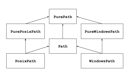
Looking at this diagram we can see that both PosixPath and WindowsPath are of the common type Path. When we make use of the Path object in our code, it determines which type of file system it is accessing and automatically implements the correct xPath object.
Note
We’re not going to worry about the pure instances of the pathlib module in this course. If you are curious you can read more on the link to Python docs above. For now, it’s probably easiest to think about the pure versions as a set of rules or specifications for implementing xPath objects, whereas the non-pure versions are concrete implementations that we can use in our programs.
For most cases, you will want to use Path whenever possible when working directly with the file system. So let’s look at some of things a Path object can do.
The code snippets we have looked at so far have instantiated or created an instance of a Path object with a directory parameter.
#files_demo.py

from pathlib import Path

p1 = Path()
p2 = Path('.')

# or

p3 = Path('c:\\users\\marks')
In the code snippet above, p1 and p2 are the same. If you do not provide a parameter to Path it will default to the current directory (e.g., ‘.’). p3 is an example of instantiating Path to a specific directory. The directory that you specify, then, will be the directory that you will work from using the variable to which you have assigned the Path object.
Exploring the Contents of a Directory
One of the more common tasks you will perform when working with the Path object is to look at the contents of a directory. We can use the iterdir function to help us with this task:
#files_demo.py

from pathlib import Path

p = Path('.') # we'll work with current directory, but feel free to add your preferred directory here.

for obj in p.iterdir():
  print(obj)
Running this code will print a Path object, stored in the obj variable, for each item in the directory used to create the p variable. Since this output will be different for each computer system, your results will vary, but you should expect to see the names of files and directories in your current working directory. If nothing prints, then make sure there are file objects in your current working directory or use a different directory when creating the Path object.
iterdir will iterate over all objects in a directory, both files and directories. So if we want to understand the type of Path object, there are two functions that can help: is_file and is_dir. Let’s see how they work.
files = 0
dirs = 0

for obj in p.iterdir():
  if obj.is_file():
		files = files + 1
  elif obj.is_dir():
    dirs = dirs + 1

print(f"There are {files} files and {dirs} in {p})
Both functions will return a boolean value indicating whether or not the Path object represents a file or directory. There are many more functions and properties of the Path object available to help understand the data it represents. We won’t cover all of them in great detail here as they all more or less operate through the same behavior. Rather, you should visit the Python docs to learn more. But, before we move on, let’s take a look at a few of the most useful properties for the work we will be doing throughout this course.
p1 = Path(".") / "temp_dir"

if not p1.exists(): # check to see if temp_dir exists
  p1.mkdir() # if temp_dir does not exist, create it

p1 = p1 / "temp_file.txt" # append a file name to the current path

if not p1.exists(): # check to see if temp_file.txt exists
  p1.touch() # if temp_file.txt does not exist, create it

print(p1.name) # get the name of the object (file name or directory name)
print(p1.suffix) # get the suffix (.py, .doc, etc) of the file object
In the code above, we have a simple program that first changes the file system path from the current working directory (“.”) to a directory called temp_dir located within the current working directory. With the update path, it then checks if temp_dir exists by calling the exists function. If it doesn’t exist, then the mkdir function is called to create the new directory. The next line performs a similar task to create the file temp_file.txt. With the updated path, it checks to see if temp_file.txt actually exists by calling the exists function. If it doesn’t exist, then the touch function is called to create it. Finally, we print two properties of the path object, name and suffix to learn more about the file. Go ahead and run this code on your system, but before you do, what do you think will be printed by those last two print statements?
One more thing, notice the use of the forward slash, /, between the instantiation of the Path object and the file name (and directory name) string. This is a syntactic shorthand for the joinpath function. Let’s update the fourth line of the program above to use joinpath:
p1 = p1.joinpath("temp_file.txt") # append a file name to the current path
Both approaches accomplish the same thing, but you might decide that using the / symbol is a little less work. Either approach works and ensures that when you combine paths they will safely work on both Windows and Posix systems. You should avoid using string concatenation on paths at all costs. For example, the following operation might work on your computer (if you are on Windows):
p1 = Path(".") + "//" + "temp_file.txt" # append a file name to the current path
But it will not work on a Posix system, removing all of the benefits of working with the Path object!
So now that we know how to locate, create, and learn about files and directories, let’s talk about how to work with the files that we find and create.
Working with Files
When writing Python programs that work with files, you will likely need to be able to read and write information to and from a file. To read or write, we must first open the file that is being used for our work. Thankfully, the Path object makes this fairly straightforward by providing an open function on file objects. Let’s continue to extend our small program from the previous section:
p1 = Path(".") / "temp_dir" / "temp_file.txt"

if p1.exists(): # check to see if temp_file exists
  f = p1.open()
  print(f.readline())
  f.close()
This very simple program opens the file represented by the Path object in the variable p1 and assigns the open file to the variable f. It then reads the first line in the file and prints the content to the shell. Finally, when all operations are complete, the file object is closed by calling the close function on the file object.
If you run this code you will find that nothing is actually printed! Assuming you have been following along, then your temp_file.txt file doesn’t have any information in it yet. So let’s add some:
p1 = Path(".") / "temp_dir" / "temp_file.txt"

if p1.exists(): # check to see if temp_file exists
  f = p1.open('w')
  f.write("Hello New File!")
  f.close()

  f = p1.open('r')
  print(f.readline())
  f.close()
The revised program above will now print the contents of the file that was added using the write command. You have likely noticed the addition of the letters w and r to the open function in the final version of the program here. “w” implies that you intend to perform a write operation with the file that is opened and “r” implies that you intend to perform a read operation. Since open defaults to read mode, if you only intend to perform a read operation, then the use of “r” is unnecessary.
Note
One consequence of opening a file in write mode is that all existing contents of the file will be deleted. If you plan on appending content to an existing file, then you will need to use the “a” parameter option when opening a file:
f = p1.open('a')
Alright, that’s it for files and file systems! The code discussed here should provide you with nearly everything you need to know to assemble a program that traverses, reads, writes, and creates files and directories in a file system. There are few operations that we have intentionally not covered (e.g., delete operations). This lecture should provide you with enough of the building blocks that, when combined with the Python documentation for the pathlib module, will allow you to identify and implement any remaining tasks on your own.
Recursion
Lecture Recording
Lecture Notes
In this lecture we are going to talk about recursion.

Let’s start with an example. Take the onion, as you might imagine every onion develops differently. They are different sizes and they have different amounts of outer and inner layers. So each time we peel a new onion, the work effort to remove all of the layers down to the core will be different. If we think of the action required to remove one outer layer of an onion as a single operation, then one onion might require 10 peel operations. Another might require 15. And another might only need 5.
So given a basket of onions to peel, as you might imagine, if we were to peel each onion by hand, that would be a lot of work!
But, perhaps we can automate the work to save us some time, effort, and the inevitable onion tears…
So let’s imagine that the onion is a Python object that we can write some code to peel.
Note
Don’t worry too much about the Onion object. You can take a look at by expanding the following section, but for now, just assume that the Onion object has a random number of layers, can remove layers one at a time, and can report whether or not it still has layers.
import random

class Onion:
    layers = 0

    def __init__(self):
        self.layers = random.randrange(5, 15)

    def removelayer(self):
        if self.layers > 0:
            self.layers -= 1

    def is_layer(self) -> bool:
       return self.layers > 0
The countlayers() function looks like a pretty good way to go about peeling the layers off of our onion object, right? In fact, it is! Although the onion is not the perfect metaphor for recursive properties, it provides us with a constrained conceptual model that we can build upon.
def countlayers():
    onions = Onion(), Onion(), Onion()
    layers = 0

    for onion in onions:
        while onion.is_layer():
            onion.removelayer()
            layers += 1

    print(layers)
Okay, so let’s talk about what we mean when we say recursive.
In programming languages, a recursive function call means that you call a function from within that same function. So you can see what that looks like in this pseudo code here:
def recurse():
    recurse()   # <- Recursive function call


def main():
    recurse()   # <- Normal function call
Take a minute and think about why the pseudo code here is problematic.
Imagine what would happen if we were to run the main function right now?
We would actually receive a RecursionError exception. Effectively what we did was put the program into an infinite loop! That’s bad. So when we write recursive functions, we need to take care that our code contains a terminal condition, something to ensure that at some point the recursive call will end.
Let’s take a look at the onion peeler again, this time we will make some modifications to apply recursive principles rather than nested loops.
def peel(onion, layer_count) -> int:
    onion.removelayer()

    if onion.is_layer():
        return peel(onion, layer_count + 1) # recursive call
    else:
        return layer_count

def countlayers_recursively():
    onions = Onion(), Onion(), Onion()
    layers = 0

    for onion in onions:
        layers +=  peel(onion, 0)

    print(layers)
So the code we have written here, is probably not the best case for demonstrating the value of recursion, but I think by approaching it this way, internalizing the goal of using recursive logic is a little easier.
Fortunately, the onion is not a very complex structure, so the advantages of recursion are less apparent here. So let’s think of another metaphor that is complex.
How about a tree?

Slightly more complex, right? So let’s say you want to count the leaves on a tree…think about how you might do that without recursion. Each branch has the possibility to contain infinite branches with infinite leaves! Of course, a real tree is constrained by physical and environmental conditions, so there are some finite bounds, but a computational tree, given enough memory, is limitless.
Let’s take a more practical look using nested lists.
Note
sum functions adapted from Alex Thornton
def simple_sum(num_list: [int]) -> int:
    total = 0

    for n in num_list:
        total += n

    return total

print(simple_sum([1,2,3,4,5,6]))

def list_sum(num_list: [[int]]) -> int:
    total = 0

    for l in num_list:
        for n in l:
            total += n

    return total

print(list_sum([[1],[2,3],[4,5,6]]))

def complex_sum(num_list: [int or [int]]) -> int:
    total = 0

    for obj in num_list:
        if type(obj) == list:
            for n in obj:
                total += n
        else:
            total += obj # if not a list, must be integer

    return total

print(complex_sum([1,2,[3,4],[5],6]))
Running each of these functions right now, is probably unnecessary. You can assume that each will return a sum of the integers passed as function parameter. But, feel free to take a minute to run each if you would like.
Rather, pay attention to the increasing complexity of each function as we increase the complexity of our list parameter. Notice how each parameter creates additional rules to take into account, and how each function requires additional logic to handle the complexity.
By the time we get to complex_sum, we are working with two nested levels and a single integer. But, like the tree with infinite branches and leaves, what happens when we need to add a third level of nested lists? How about a fourth level?
This is where recursion becomes truly invaluable. We can replace all three of the sum functions here and any additional functions required to support deeper nesting, with a single recursive function.
def recursive_sum(nested_list) -> int:
    total = 0

    for obj in nested_list:
        if type(obj) == list:
            total += recursive_sum(obj)  # <- recursive call
        else:
            total += obj # if not a list, must be integer

    return total

print(recursive_sum([1,2,3,4,5,6]))
print(recursive_sum([[1],[2,3],[4,5,6]]))
print(recursive_sum([1,2,[3,4],[5],6]))
Pretty cool, right?
Okay, one final thought. Guess what else is like a tree with branches or an infinitely nestable list (toggle to reveal the answer)?
The computer file system! (ahem, a1)